EndTailImputer#
The EndTailImputer() replaces missing data with a value at the end of the distribution.
The value can be determined using the mean plus or minus a number of times the standard
deviation, or using the inter-quartile range proximity rule. The value can also be
determined as a factor of the maximum value.
You decide whether the missing data should be placed at the right or left tail of the variable distribution.
In a sense, the EndTailImputer() “automates” the work of the
ArbitraryNumberImputer() because it will find automatically “arbitrary values”
far out at the end of the variable distributions.
EndTailImputer() works only with numerical variables. You can impute only a
subset of the variables in the data by passing the variable names in a list. Alternatively,
the imputer will automatically select all numerical variables in the train set.
Below a code example using the House Prices Dataset (more details about the dataset here).
First, let’s load the data and separate it into train and test:
import numpy as np
import pandas as pd
import matplotlib.pyplot as plt
from sklearn.model_selection import train_test_split

from feature_engine.imputation import EndTailImputer

# Load dataset
data = pd.read_csv('houseprice.csv')

# Separate into train and test sets
X_train, X_test, y_train, y_test = train_test_split(
                                    data.drop(['Id', 'SalePrice'], axis=1),
                                    data['SalePrice'],
                                    test_size=0.3,
                                    random_state=0,
                                    )
Now we set up the EndTailImputer() to impute in this case only 2 variables
from the dataset. We instruct the imputer to find the imputation values using the mean
plus 3 times the standard deviation as follows:
# set up the imputer
tail_imputer = EndTailImputer(imputation_method='gaussian',
                          tail='right',
                          fold=3,
                          variables=['LotFrontage', 'MasVnrArea'])
# fit the imputer
tail_imputer.fit(X_train)
With fit, the EndTailImputer() learned the imputation values for the indicated
variables and stored it in one of its attributes. We can now go ahead and impute both
the train and the test sets.
# transform the data
train_t= tail_imputer.transform(X_train)
test_t= tail_imputer.transform(X_test)
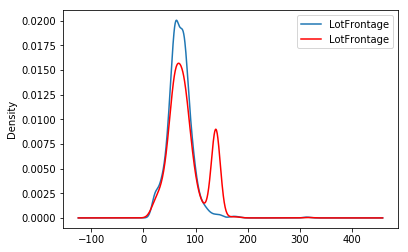
Note that after the imputation, if the percentage of missing values is relatively big, the variable distribution will differ from the original one (in red the imputed variable):
fig = plt.figure()
ax = fig.add_subplot(111)
X_train['LotFrontage'].plot(kind='kde', ax=ax)
train_t['LotFrontage'].plot(kind='kde', ax=ax, color='red')
lines, labels = ax.get_legend_handles_labels()
ax.legend(lines, labels, loc='best')
Additional resources#
In the following Jupyter notebook you will find more details on the functionality of the
CategoricalImputer(), including how to select numerical variables automatically,
how to impute with the most frequent category, and how to impute with a used defined
string.
For more details about this and other feature engineering methods check out these resources:

Feature Engineering for Machine Learning#
Or read our book:

Python Feature Engineering Cookbook#
Both our book and course are suitable for beginners and more advanced data scientists alike. By purchasing them you are supporting Sole, the main developer of Feature-engine.