ArcsinTransformer#
The ArcsinTransformer() applies the arcsin transformation to
numerical variables.
The arcsine transformation, also called arcsin square root transformation, or angular transformation, takes the form of arcsin(sqrt(x)) where x is a real number between 0 and 1.
The arcsin square root transformation helps in dealing with probabilities, percentages, and proportions.
The ArcsinTransformer() only works with numerical variables with values
between 0 and 1. If the variable contains a value outside of this range, the
transformer will raise an error.
Example#
Let’s load the breast cancer dataset from scikit-learn and separate it into train and test sets.
import numpy as np
import pandas as pd
import matplotlib.pyplot as plt
from sklearn.model_selection import train_test_split
from sklearn.datasets import load_breast_cancer

from feature_engine.transformation import ArcsinTransformer

#Load dataset
breast_cancer = load_breast_cancer()
X = pd.DataFrame(breast_cancer.data, columns=breast_cancer.feature_names)
y = breast_cancer.target

# Separate data into train and test sets
X_train, X_test, y_train, y_test = train_test_split(X, y, random_state=0)
Now we want to apply the arcsin transformation to some of the variables in the dataframe. These variables values are in the range 0-1, as we will see in coming histograms.
First, let’s make a list with the variable names:
vars_ = [
  'mean compactness',
  'mean concavity',
  'mean concave points',
  'mean fractal dimension',
  'smoothness error',
  'compactness error',
  'concavity error',
  'concave points error',
  'symmetry error',
  'fractal dimension error',
  'worst symmetry',
  'worst fractal dimension']
Now, let’s set up the arscin transformer to modify only the previous variables:
# set up the arcsin transformer
tf = ArcsinTransformer(variables = vars_)

# fit the transformer
tf.fit(X_train)
The transformer does not learn any parameters when applying the fit method. It does check however that the variables are numericals and with the correct value range.
We can now go ahead and transform the variables:
# transform the data
train_t = tf.transform(X_train)
test_t = tf.transform(X_test)
And that’s it, now the variables have been transformed with the arscin formula.
Finally, let’s make a histogram for each of the original variables to examine their distribution:
# original variables
X_train[vars_].hist(figsize=(20,20))
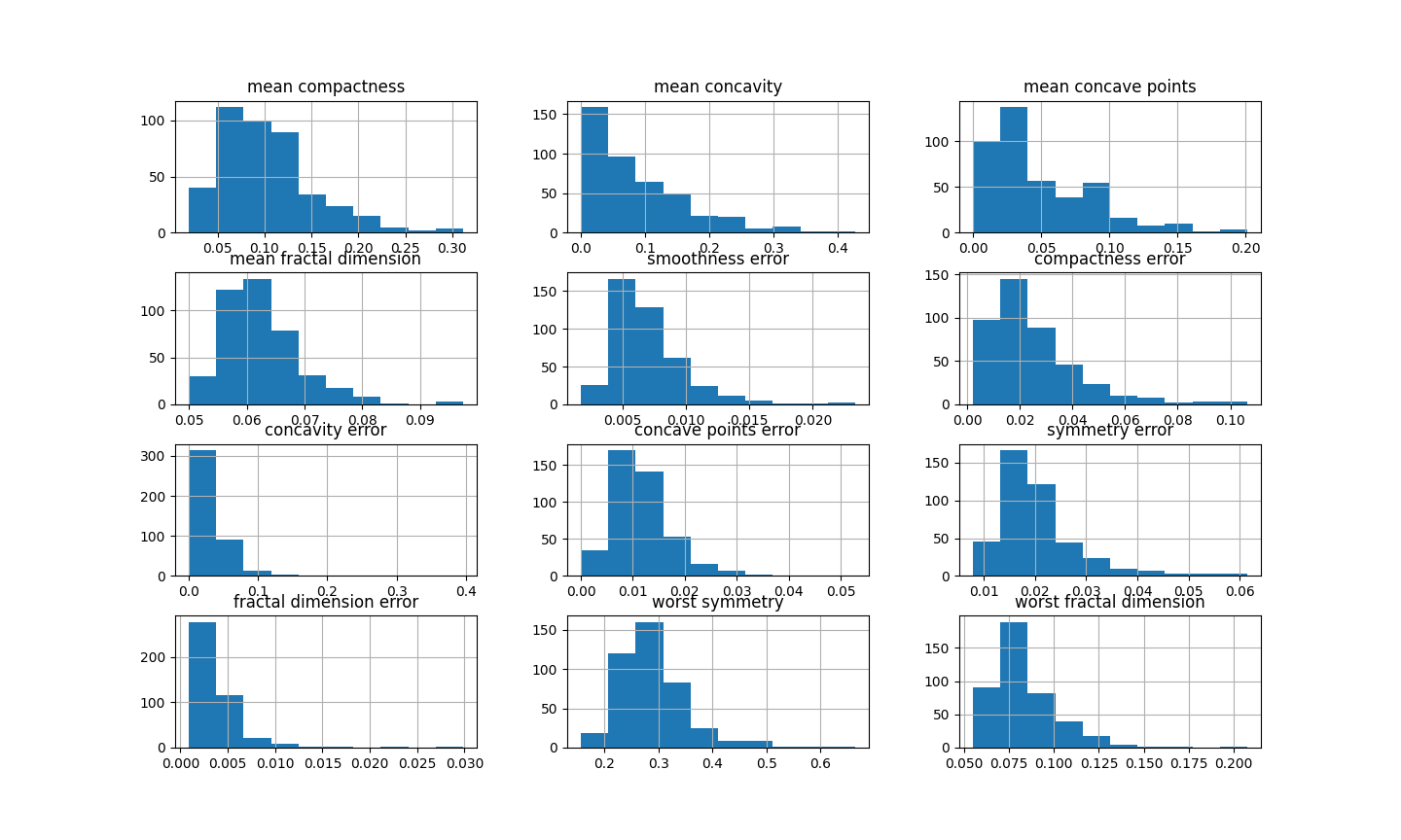
You can see in the previous image that many of the variables are skewed. Note however, that all variables had values between 0 and 1.
Now, let’s examine the distribution after the transformation:
# transformed variable
train_t[vars_].hist(figsize=(20,20))
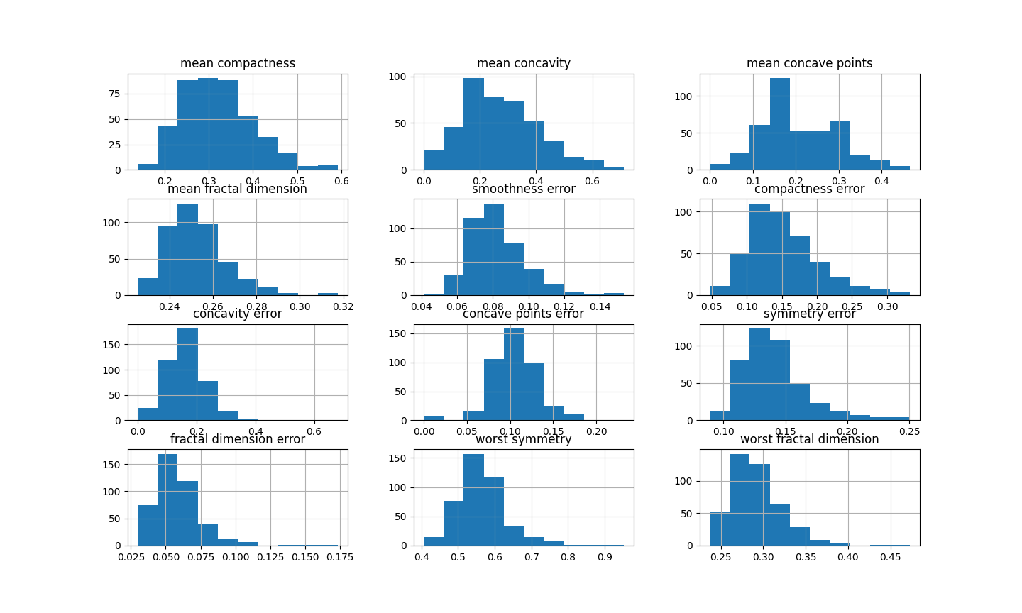
You can see in the previous image that many variables have after the transformation a more Gaussian looking shape.
More details#
For more details about this and other feature engineering methods check out these resources:
Feature engineering for machine learning, online course.