CyclicalFeatures#
Some features are inherently cyclical. Clear examples are time features, i.e., those features derived from datetime variables like the hours of the day, the days of the week, or the months of the year.
But that’s not the end of it. Many variables related to natural processes are also cyclical, like, for example, tides, moon cycles, or solar energy generation (which coincides with light periods, which are cyclical).
In cyclical features, higher values of the variable are closer to lower values. For example, December (12) is closer to January (1) than to June (6).
How can we convey to machine learning models like linear regression the cyclical nature of the features?
In the article “Advanced machine learning techniques for building performance simulation,” the authors engineered cyclical variables by representing them as (x,y) coordinates on a circle. The idea was that, after preprocessing the cyclical data, the lowest value of every cyclical feature would appear right next to the largest value.
To represent cyclical features in (x, y) coordinates, the authors created two new features, deriving the sine and cosine components of the cyclical variable. We can call this procedure “cyclical encoding.”
Cyclical encoding#
The trigonometric functions sine and cosine are periodic and repeat their values every 2 pi radians. Thus, to transform cyclical variables into (x, y) coordinates using these functions, first we need to normalize them to 2 pi radians.
We achieve this by dividing the variables’ values by their maximum value. Thus, the two new features are derived as follows:
var_sin = sin(variable * (2. * pi / max_value))
var_cos = cos(variable * (2. * pi / max_value))
In Python, we can encode cyclical features by using the Numpy functions sin and cos:
import numpy as np

X[f"{variable}_sin"] = np.sin(X["variable"] * (2.0 * np.pi / X["variable"]).max())
X[f"{variable}_cos"] = np.cos(X["variable"] * (2.0 * np.pi / X["variable"]).max())
We can also use Feature-Engine to automate this process.
Cyclical encoding with Feature-engine#
CyclicalFeatures() creates two new features from numerical variables to better
capture the cyclical nature of the original variable. CyclicalFeatures() returns
two new features per variable, according to:
var_sin = sin(variable * (2. * pi / max_value))
var_cos = cos(variable * (2. * pi / max_value))
where max_value is the maximum value in the variable, and pi is 3.14…
Example#
In this example, we obtain cyclical features from the variables days of the week and months. We first create a toy dataframe with the variables “days” and “months”:
import pandas as pd
from feature_engine.creation import CyclicalFeatures

df = pd.DataFrame({
    'day': [6, 7, 5, 3, 1, 2, 4],
    'months': [3, 7, 9, 12, 4, 6, 12],
    })
Now we set up the transformer to find the maximum value of each variable automatically:
cyclical = CyclicalFeatures(variables=None, drop_original=False)

X = cyclical.fit_transform(df)
The maximum values used for the transformation are stored in the attribute
max_values_:
print(cyclical.max_values_)
{'day': 7, 'months': 12}
Let’s have a look at the transformed dataframe:
print(X.head())
We can see that the new variables were added at the right of our dataframe.
   day  months       day_sin   day_cos    months_sin    months_cos
0    6       3 -7.818315e-01  0.623490  1.000000e+00  6.123234e-17
1    7       7 -2.449294e-16  1.000000 -5.000000e-01 -8.660254e-01
2    5       9 -9.749279e-01 -0.222521 -1.000000e+00 -1.836970e-16
3    3      12  4.338837e-01 -0.900969 -2.449294e-16  1.000000e+00
4    1       4  7.818315e-01  0.623490  8.660254e-01 -5.000000e-01
We set the parameter drop_original to False, which means that we keep the original
variables. If we want them dropped after the feature creation, we can set the parameter
to True.
We can now use the new features, which convey the cyclical nature of the data, to train machine learning algorithms, like linear or logistic regression, among others.
Finally, we can obtain the names of the variables of the transformed dataset as follows:
cyclical.get_feature_names_out()
This returns the name of all the variables in the final output, original and and new:
['day', 'months', 'day_sin', 'day_cos', 'months_sin', 'months_cos']
Cyclical feature visualization#
We now know how to convert cyclical variables into (x, y) coordinates of a circle by using the sine and cosine functions. Let’s now carry out some visualizations to better understand the effect of this transformation.
Let’s create a toy dataframe:
import pandas as pd
import matplotlib.pyplot as plt

df = pd.DataFrame([i for i in range(24)], columns=['hour'])
Our dataframe looks like this:
df.head()

   hour
0     0
1     1
2     2
3     3
4     4
Let’s now compute the sine and cosine features:
cyclical = CyclicalFeatures(variables=None)

df = cyclical.fit_transform(df)

print(df.head())
These are the sine and cosine features that represent the hour:
   hour  hour_sin  hour_cos
0     0  0.000000  1.000000
1     1  0.269797  0.962917
2     2  0.519584  0.854419
3     3  0.730836  0.682553
4     4  0.887885  0.460065
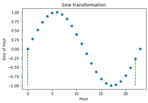
Let’s now plot the hour variable against its sine transformation. We add perpendicular lines to flag the hours 0 and 22.
plt.scatter(df["hour"], df["hour_sin"])

# Axis labels
plt.ylabel('Sine of hour')
plt.xlabel('Hour')
plt.title('Sine transformation')

plt.vlines(x=0, ymin=-1, ymax=0, color='g', linestyles='dashed')
plt.vlines(x=22, ymin=-1, ymax=-0.25, color='g', linestyles='dashed')
After the transformation using the sine function, we see that the new values for the hours 0 and 22 are closer to each other (follow the dashed lines), which was the expectation:
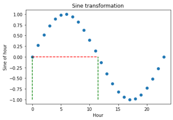
The problem with trigonometric transformations, is that, because they are periodic, 2 different observations can also return similar values after the transformation. Let’s explore that:
plt.scatter(df["hour"], df["hour_sin"])

# Axis labels
plt.ylabel('Sine of hour')
plt.xlabel('Hour')
plt.title('Sine transformation')

plt.hlines(y=0, xmin=0, xmax=11.5, color='r', linestyles='dashed')

plt.vlines(x=0, ymin=-1, ymax=0, color='g', linestyles='dashed')
plt.vlines(x=11.5, ymin=-1, ymax=0, color='g', linestyles='dashed')
In the plot below, we see that the hours 0 and 11.5 obtain very similar values after the sine transformation. So how can we differentiate them?
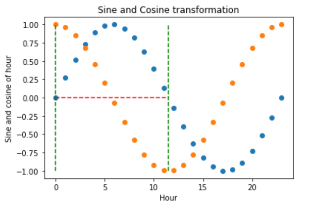
To fully code the information of the hour, we must use the sine and cosine trigonometric transformations together. Adding the cosine function, which is out of phase with the sine function, breaks the symmetry and assigns a unique codification to each hour.
Let’s explore that:
plt.scatter(df["hour"], df["hour_sin"])
plt.scatter(df["hour"], df["hour_cos"])

# Axis labels
plt.ylabel('Sine and cosine of hour')
plt.xlabel('Hour')
plt.title('Sine and Cosine transformation')


plt.hlines(y=0, xmin=0, xmax=11.5, color='r', linestyles='dashed')

plt.vlines(x=0, ymin=-1, ymax=1, color='g', linestyles='dashed')
plt.vlines(x=11.5, ymin=-1, ymax=1, color='g', linestyles='dashed')
The hour 0, after the transformation, takes the values of sine 0 and cosine 1, which makes it different from the hour 11.5, which takes the values of sine 0 and cosine -1. In other words, with the two functions together, we are able to distinguish all observations within our original variable.
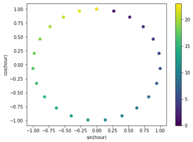
Finally, let’s vizualise the (x, y) circle coordinates generated by the sine and cosine features.
fig, ax = plt.subplots(figsize=(7, 5))
sp = ax.scatter(df["hour_sin"], df["hour_cos"], c=df["hour"])
ax.set(
    xlabel="sin(hour)",
    ylabel="cos(hour)",
)
_ = fig.colorbar(sp)
That’s it, you now know how to represent cyclical data through the use of trigonometric functions and cyclical encoding.
Additional resources#
For tutorials on how to create cyclical features, check out the following courses:

Feature Engineering for Machine Learning#

Feature Engineering for Time Series Forecasting#
For a comparison between one-hot encoding, ordinal encoding, cyclical encoding and spline encoding of cyclical features check out the following sklearn demo.
Check also these Kaggle demo on the use of cyclical encoding with neural networks: